Quickstart
Installation
If you have not installed Python and setup a project, follow this guide Installing Python.
If you have not already installed PyOptEx, first install it using pip:
(.venv) $ pip install pyoptex
Analyze your first dataset
Create a predetermined linear model is very easy. The full Python script for this example can be found at simple_model.py.
Let us assume that we have 200 random observations from a process with three continuous variables A, B, and C.
Start with the necessary imports
>>> import numpy as np
>>> import pandas as pd
>>>
>>> from pyoptex.utils import Factor
>>> from pyoptex.utils.model import model2Y2X, partial_rsm_names
>>> from pyoptex.analysis import SimpleRegressor
>>> from pyoptex.analysis.utils.plot import plot_res_diagnostics
Next, we define the factors in our simulation
>>> # Define the factors
>>> factors = [
>>>     Factor('A'), Factor('B'), Factor('C')
>>> ]
Then, we define the data for our simulation
>>> # The number of random observations
>>> N = 200
>>>
>>> # Define the data
>>> data = pd.DataFrame(np.random.rand(N, 3) * 2 - 1, columns=[str(f.name) for f in factors])
>>> data['Y'] = 2*data['A'] + 3*data['C'] - 4*data['A']*data['B'] + 5\
>>>                 + np.random.normal(0, 1, N)
Just like in design of experiments, we define the model we want to fit. In this case, it is a response surface model (or a full quadratic model containing the intercept and all main effects, interactions, and quadratic effects).
First, we create a matrix representation of our model using the
partial_rsm_names function.
Then, we convert this model to a function which transforms Y to X using the
model2Y2X function.
>>> model = partial_rsm_names({str(f.name): 'quad' for f in factors})
>>> Y2X = model2Y2X(model, factors)
Finally, we create the
SimpleRegressor
and fit it to the data
>>> regr = SimpleRegressor(factors, Y2X)
>>> regr.fit(data.drop(columns='Y'), data['Y'])
To analyze the results, we can do a few things. First, we can print the summary of the fit which includes the coefficients of the normalized data, the scale of the data, etc.
>>> print(regr.summary())
                            OLS Regression Results
==============================================================================
Dep. Variable:                      y   R-squared:                       0.850
Model:                            OLS   Adj. R-squared:                  0.843
Method:                 Least Squares   F-statistic:                     119.5
Date:                Tue, 07 Jan 2025   Prob (F-statistic):           2.59e-73
Time:                        09:57:03   Log-Likelihood:                -94.165
No. Observations:                 200   AIC:                             208.3
Df Residuals:                     190   BIC:                             241.3
Df Model:                           9
Covariance Type:            nonrobust
==============================================================================
                 coef    std err          t      P>|t|      [0.025      0.975]
------------------------------------------------------------------------------
const          0.0791      0.065      1.213      0.226      -0.049       0.208
x1             0.7721      0.049     15.677      0.000       0.675       0.869
x2            -0.0519      0.048     -1.090      0.277      -0.146       0.042
x3             1.1409      0.047     24.225      0.000       1.048       1.234
x4            -1.5120      0.084    -17.989      0.000      -1.678      -1.346
x5            -0.0666      0.086     -0.774      0.440      -0.236       0.103
x6             0.0065      0.076      0.085      0.933      -0.144       0.157
x7             0.0230      0.096      0.238      0.812      -0.167       0.213
x8            -0.0686      0.092     -0.743      0.458      -0.251       0.114
x9             0.0377      0.092      0.410      0.683      -0.144       0.219
==============================================================================
Omnibus:                        1.938   Durbin-Watson:                   1.839
Prob(Omnibus):                  0.379   Jarque-Bera (JB):                1.933
Skew:                           0.236   Prob(JB):                        0.380
Kurtosis:                       2.900   Cond. No.                         4.93
==============================================================================
We can also print the prediction formula using
model_formula.
Note
model_formula
is only possible if we have created Y2X using
model2Y2X
as done in this example. Otherwise, use
formula
and specify your own labels.
Warning
The prediction formula is based on the encoded model. Make sure
to first normalize the data between -1 and 1, and encode the
categorical variables. See
formula
for the complete warning.
>>> print(regr.model_formula(model=model))
0.079 * cst + 0.772 * A + -0.052 * B + 1.141 * C + -1.512 * A * B + -0.067 * A * C + 0.006 * B * C + 0.023 * A^2 + -0.069 * B^2 + 0.038 * C^2
Prediction is as easy as calling .predict()
>>> data['pred'] = regr.predict(data.drop(columns='Y'))
Finally, to investigate how good it fits, we introduced
plot_res_diagnostics
>>> plot_res_diagnostics(
>>>     data, y_true='Y', y_pred='pred',
>>>     textcols=[str(f.name) for f in factors],
>>> ).show()
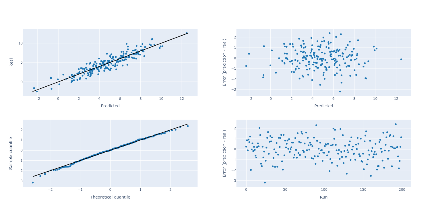
The upper left plot indicates the predicted vs. fit plot. Ideally, all elements are on the black diagonal. The upper right plot provides the error vs. the prediction. A positive errors means an overprediction. In case a trend or divergence is observed, it could indicate a lack of fit. Ideally, the data is normally distributed around the x-axis, in a rectangular block. The lower left plot is the quantile-quantile distribution of the errors against a normal distribution. If all points are on the black diagonal, the errors are normally distributed. Significant deviations may indicate outliers. The lower right plot is the error vs. the run. Again, a positive error means an overprediction. This plot is useful to analyze potential time trends in the data if your data is sorted in time.