Customization
Custom models
In Create your first design, we created a response surface model
using the partial_rsm_names
function. While, for most scenarios, a response surface model is more than
complex enough, not all scenarios require such a model.
Instead of generating the model from the different factors, we can also manually define the desired model. A model is defined as a matrix where each column represents a factor, and each row represents a term. The value in each cell of the matrix represents a power. For example, assume that the factor names are x1, x2, and x3
The row [0, 0, 0] represents \(x_1^0 \cdot x_2^0 \cdot x_3^0 = 1\), the intercept.
The row [1, 0, 0] represents \(x_1^1 \cdot x_2^0 \cdot x_3^0 = x_1\).
The row [1, 1, 0] represents \(x_1^1 \cdot x_2^1 \cdot x_3^0 = x_1 x_2\).
The row [1, 2, 0] represents \(x_1^1 \cdot x_2^2 \cdot x_3^0 = x_1 x_2^2\).
Such a design can be manually created as a csv or in excel and read using pandas
>>> import pandas as pd
>>> model = pd.read_csv('...')
Or
>>> model = pd.read_excel('...')
Finally, the model can be transformed to a callable using the same
model2Y2X call
>>> Y2X = model2Y2X(model, factors)
If the user requires an even more complex linear model which can not be expressed as a product of powers, the user can directly implement the Y2X function. For example, assume the user wants to generate a design for the linear model \(y = \beta_0 + \beta_1 x + \beta_2 sin(x) + \epsilon\)
>>> def Y2X(Y)
>>>     X = np.stack((
>>>         np.ones(len(Y)),
>>>         Y[0]
>>>         np.sin(Y[0]),
>>>     ), axis=1)
>>>     return X
Warning
You are creating an internal function here. The input Y is a 2D numpy array which has the categorical factors encoded and all factors normalized to between -1 and 1. This is important when specifying the column you transform from Y.
Custom metrics
Metrics or optimization criteria can also be fully customized, which can be interesting for researchers who which to develop such a new criterion. The method to create a new metric depends slightly on which algorithm it targets
Fixed structure design
The easiest way to create a new criterion is to ignore any potential
update formulas. First, import the interface
which should be extended
>>> from pyoptex.doe.fixed_structure.metric import Metric
The user is required to implement the
call function.
The example below implements the D-optimal criterion for the first
set of a-priori variance ratios.
>>> class CustomMetric(Metric):
>>>    def call(self, Y, X, params):
>>>        assert len(params.Vinv) == 1, 'This criterion only works with one set of a-priori variance ratios'
>>>
>>>        # Compute information matrix
>>>        M = X.T @ params.Vinv[0] @ X
>>>
>>>        # Compute D-optimality
>>>        return np.power(np.maximum(np.linalg.det(M), 0), 1/X.shape[1])
We first compute the information matix, and then compute \(|M|^{1/p}\), with p the number of parameters in the linear model.
Note
Computing the information is based on the first Vinv, which represents the inverse of the observation covariance matrix. Multiple sets of variance ratios can be provided by the user. More information in Bayesian a-priori variances.
If the criterion requires some pre-initialization, this can be coded in the
preinint function.
For instance, the I-optimal criterion is required to compute the moments matrix.
Warning
The above examples never considered any potential covariate function such as a time trend. Without update formulas, the call function should first call
>>> Y, X = self.cov(Y, X)
Splitk-plot design
Splitk-plot designs are specialized versions of the fixed structure designs. They permit the use of update formulas.
The best way to create a splitk-plot metric is to extend from a fixed_structure metric, such as the CustomMetric above, as follows
>>> from pyoptex.doe.fixed_structure.splitk_plot import SplitkPlotMetricMixin
>>>
>>> class CustomSplitkMetric(SplitkPlotMetricMixin, CustomMetric):
>>>     pass
By default, the metric does not yet use update formulas. In order to
do so, the user should implement three additional functions:
_init,
_update,
and _accepted.
The first function occurs after the initialization of a random design. For example in D-optimality, the user can initialize the inverse of the information matrix using.
>>> def _init(self, Y, X, params):
>>>     M = X.T @ params.Vinv @ X
>>>     self.Minv = np.linalg.inv(M)
Next, whenever an update is made to a coordinate from the coordinate-exchange
algorithm, the _update
function is called. This function computes the update to the metric, given the
update to the design.
>>> def _update(self, Y, X, params, update):
>>>     # Compute U, D update
>>>     self.U, self.D = compute_update_UD(
>>>         update.level, update.grp, Xi_old, X,
>>>         params.plot_sizes, params.c, params.thetas, params.thetas_inv
>>>     )
>>>
>>>     # Compute change in determinant
>>>     du, self.P = det_update_UD(self.U, self.D, self.Minv)
>>>     if du > 0:
>>>         # Compute power
>>>         duu = np.power(np.prod(du), 1/(X.shape[1] * len(self.Minv)))
>>>
>>>         # Return update as addition
>>>         metric_update = (duu - 1) * update.old_metric
>>>     else:
>>>         metric_update = -update.old_metric
>>>
>>>     return metric_update
These formulas rely on the fact that any coordinate update to the
information matrix can be expressed as \(M^* = M + U^T D U\). In order to
do so, a subfunction was developed which creates the matrices U and D.
Next, we check for an update to the determinant using
det_update_UD.
Finally, we determine what the update to the D-criterion would be in case the
proposed coordinate-exchange would be applied. For I-optimality, the
subfunction inv_update_UD_no_P
can be used.
If the update is accepted by the coordinate-exchange algorithm, the
_accepted function
is called, and we should update our internal caches. In the D-optimality case,
we should update our Minv parameter.
>>> def _accepted(self, Y, X, params, update):
>>>     try:
>>>         self.Minv -= inv_update_UD(self.U, self.D, self.Minv, self.P)
>>>     except np.linalg.LinAlgError as e:
>>>         warnings.warn('Update formulas are very unstable for this problem, try rerunning without update formulas', RuntimeWarning)
>>>         raise e
Note that some times, update formulas of the above form can be unstable.
In such a case, the design can be created without update formulas by passing
use_formulas=False to create_splitk_plot_design
Warning
The above update formulas also never considered any covariate function. The exact implementation depends on the criterion.
Cost-optimal design
The creation of a metric for the cost-optimal algorithm
is slightly different. First, import the
interface
which should be extended
>>> from pyoptex.doe.cost_optimal.metric import Metric
The user should extend the metric and implement the
call
function. Here, we recreate the D-optimality criterion.
>>> class CustomMetric(Metric):
>>>    def call(self, Y, X, Zs, Vinv, costs):
>>>        assert len(Vinv) == 1, 'This criterion only works with one set of a-priori variance ratios'
>>>
>>>         # Compute the information matrix
>>>         M = X.T @ Vinv[0] @ X
>>>
>>>         # Compute determinant
>>>         return np.power(np.maximum(np.linalg.det(M), 0), 1/X.shape[1])
We first compute the information matix, and then compute \(|M|^{1/p}\), with p the number of parameters in the linear model.
Note
Computing the information is based on the first Vinv, which represents the inverse of the observation covariance matrix. Multiple sets of variance ratios can be provided by the user. More information in Bayesian a-priori variances.
In case the user wants to perform any initialization to the metric, such
as computing the moments matrix for the I-optimal criterion, he or she
can do so in the init
function.
Warning
The above examples never considered any potential covariate function such as a time trend. The call function should first call
>>> Y, X, Zs, Vinv = self.cov(Y, X, Zs, Vinv, costs)
Custom cost functions
Custom cost functions provide maximum flexibility to generate a design specifically tailored to your problem. Every design is limited by a fixed number of resource consumptions, also referred to as costs. Creating a custom cost function is extremely easy.
First, import the necessary decorator.
>>> from pyoptex.doe.cost_optimal.cost import cost_fn
Single cost function
Then, the user can specify any function to compute the costs of design Y. For example, assume we are creating cheese, and we want to know the ideal amount of milk. Each run consumes a certain amount of milk, but the total amount of milk for the entire experiment is limited. Each factor can consume between 2 and 5 liters of milk, and we have a total of 100 liters available.
>>> # For reference
>>> factors = [
>>>     Factor(name='milk', type='continuous', grouped=False, min=2, max=5)
>>>     ...
>>> ]
>>> milk_budget = 100
>>> @cost_fn
>>> def cost_milk(Y):
>>>    consumption = Y['milk']
>>>    return [(consumption, milk_budget, np.arange(len(Y)))]
The cost function is a function that takes a denormalized design as an input, and returns one or more costs. Here, we only consider the milk consumption. The function should return a list of tuples with every tuple representing a different cost. Each tuple then consists of:
An array of consumptions. It should return a value for every affected run. Here, every run consumes milk, so we return one value per run. The value itself is then the exact consumption.
The available budget. In this case 100 liters.
The affected run indices. This is mostly used when multiple resource constraints are imposed simultaneously as is explained later. This array should be of the same size as the array of consumptions.
Note
When dealing with transition costs, the cost of a transition may be assigned to either run in addition to the execution cost such as the milk consumption.
Note
The cost function returns a denormalized dataframe by default. However, such a conversion requires a lot of computational power. If possible, attempt to optimize it using the tips in Costs.
Multiple cost functions
When dealing with multiple resource constraints, multiple tuples may be returned
from the cost function. Another option to combine cost functions is to use
combine_costs.
Computing multiple costs simultaneously often offers a computational advantage,
whereas splitting them creates a development advantage.
Subcosts
Note that the number of resource constraints can vary with the design. There is no limit on the number of resource constraints. It also does not have to apply to the entire experiment. Using the third element in the tuple, the user can specify to which runs the constraint applies.
Factor level constraints
Some times, certain combinations of factor levels are impossible. These impossible combinations can be accounted for by a constraints function. The function is expressed as a script which should return true if the constraints are violated (by default, or if exclude=True) or return true if the constraints are met (if exclude=False).
For example, when factor A is L1, B cannot be smaller than 2
>>> constraints = parse_constraints_script(
>>>     f'(`A` == "L1") & (`B` < 2)', factors
>>> )
or inversly, when factor A is L1, B must be larger than or equal to 2
>>> constraints = parse_constraints_script(
>>>     f'(`A` == "L1") & (`B` >= 2)', factors
>>>     exclude=False
>>> )
These constraints should be added to the
FunctionSet
via the constraints parameter in
default_fn
Covariates
Covariates are factors which are not controllable, but are quantifiable upfront and expected to be important. Such variables, or additional random effects, can be added by means of a covariate function. The exact interface depends on which algorithm the covariate function targets.
The covariate function is added as a parameter to the criterion. Assume the covariate function is called cov.
>>> metric = Dopt(cov=cov)
An example of a preimplemented covariate function is a
time trend (splitk plot)
>>> metric = Dopt(cov=cov_time_trend(5, 20))
Note
The inputs of the covariate functions are encoded design matrices.
Fixed structure design
A covariate function is a function which alters the design and model matrix before computing the optimization criterion. For example, a time trend can be added as follows. Assume that we want a time trend for a design with 20 runs, which are spread over 5 days (or 5 distinct time points).
>>> nruns = 20
>>> ntime = 5
>>> time_array = np.repeat(np.linspace(-1, 1, ntime), nruns//ntime).reshape(-1, 1)
>>>
>>> def cov(Y, X, random=False, subset=slice(None, None)):
>>>     # Extract time
>>>     if random:
>>>         t = np.expand_dims(np.random.rand(Y.shape[0]) * 2 - 1, 1)
>>>     else:
>>>         t = time_array[subset]
>>>
>>>     # Augment Y and X
>>>     Y = np.concatenate((Y, t), axis=1)
>>>     X = np.concatenate((X, t), axis=1)
>>>     return Y, X
First, we compute the time factor values in time_array. Next, we define the covariate function. It takes the design and model matrix as an input and returns a time-augmented version. Let us first consider when random = False. In this case, we select the desired subset of the time array and augment both the design matrix and the model matrix with a linear time trend.
However, when random = True, we generate a random vector as augmentation. The random parameter is used to augment random samples such as those required to compute the moments matrix in the I-optimality criterion. In short, the random parameters specifies whether to the samples should be augmented completely randomly, or predetermined.
Cost-optimal design
The cost-optimal covariate function is pretty similar to the above. Let us reconsider the example of a time trend.
>>> ntime = 60
>>>
>>> def cov(Y, X, Zs, Vinv, costs, random=False):
>>>     # Define time array
>>>     if random:
>>>         t = np.random.rand(Y.shape[0]) * 2 - 1
>>>     else:
>>>         cum_cost = np.cumsum(costs[0][0])
>>>         t = np.floor_divide(cum_cost, time)
>>>         t = t / t[-1] * 2 - 1
>>>
>>>     # Concatenate time array
>>>     Y = np.concatenate((Y, t[:, np.newaxis]), axis=1)
>>>     X = np.concatenate((X, t[:, np.newaxis]), axis=1)
>>>
>>>     return Y, X, Zs, Vinv
Because in the cost-optimal design the number of runs continuously changes, we cannot precompute the the time array as before. However, one of the cost functions can be time. By taking np.cumsum(costs[0][0]), we know the current time at every run and can decide how to divide the time trend. In this example an additional time point is added for every hour (assuming the cost is expressed in minutes). The random parameter again specifies whether the augmentation should be for random samples, such as those used to compute the moments matrix in I-optimality, or for the actual design.
In contrast to a fixed structure design, the covariate function of
a cost-optimal design can also add additional random effects by altering
Zs and Vinv. Look at cov_block
on how to add an additional blocking effect based on the cumulative cost (e.g. time).
Design augmentation
Designs can be augmented in many ways by specifying a prior design.
Fixed structure design
Warning
This is yet to be implemented for generic, fixed structure designs.
Splitk-plot design
In splitk-plot designs, a prior should itself be a splitk-plot design. For example, assume one cateforical factor A and two continuous factors B and C.
>>> prior = (
>>>     pd.DataFrame([
>>>         ['L1', 0, 2],
>>>         ['L1', 1, 5],
>>>         ['L2', -1, 3.5],
>>>         ['L2', 0, 2]
>>>     ], columns=['A', 'B', 'C']),
>>>     [Plot(level=0, size=2), Plot(level=1, size=2)]
>>> )
The prior is a tuple with as the first element the denormalized prior dataframe.
The second element is a list of Plot
objects defining the structure of the prior design. For example, the above prior is
a split-plot design with 2 whole plots, and two runs per whole plot.
We can now use the
create_splitk_plot_design
to augment this design to any other splitk-plot design. For example,
augmenting to 4 whole plots with 2 runs per whole plot simply adds 2 additional
whole plots.
Augmenting to a design with 3 whole plots and 3 runs per plot will augment to the following design where each empty cell will be optimized.
A |
B |
C |
|---|---|---|
L1 |
0 |
2 |
L1 |
1 |
5 |
L1 |
||
L2 |
-1 |
3.5 |
L2 |
0 |
2 |
L2 |
||
Such an augmentation can be particularly useful in the event maybe more runs than anticipated can be performed for each setting of the hard-to-change factors.
Cost-optimal design
Augmenting a cost-optimal design can only be done at the end. Any new runs are appended to the prior. The prior is simply a dataframe
>>> prior = pd.DataFrame([['L1', 0, 2]], columns=['A', 'B', 'C'])
Such a dataframe can be read from a csv or an excel.
Custom categorical encoding
Optimizing for a design with categorical factors requires encoding these factors. Every categorical factor with N levels requires N-1 dummy columns in the design matrix. By default, effect encoding is applied. The first level is encoded as [1, 0, 0, …], the second as [0, 1, 0, …], and so on. Finally, the last level is encoded as [-1, -1, -1, …].
However, the user can also specify a custom encoding in the coords parameter when specifing a factor. For example
>>> factor = Factor(
>>>     name='A', type='categorical',
>>>     levels=['L1', 'L2', 'L3'],
>>>     coords=np.array([
>>>         [1, 0],
>>>         [0, 1],
>>>         [0, 0],
>>>     ])
>>> )
uses dummy encoding relative to the third level.
Discrete numerical factors
By default, every continuous factor is discretized to the normalized levels [-1, 0, 1], indicating, low, mid, and high respecitvely. However, in some scenarios, a higher degree of discretization is necessary or desirable. In this case, the user can simply specify them as values between the min and max.
>>> factor = Factor(
>>>     name='C', type='continuous',
>>>     min=2, max=5,
>>>     levels=np.linspace(2, 5, 10),
>>> )
The above uses 10 equidistant levels for the continuous factor instead of three.
Bayesian a-priori variances
When dealing with random effects, the user must make an estimate about the ratio between the random effect and the random errors. Most often, the user has no idea what these should be. A common solution is to set the ratio to 1, meaning the variance of the random effects is the same as the variance of the random errors.
Note
It is better to overestimate than underestimate the variance ratios.
However, a second solution originates from a Bayesian approach. The user can specify multiple variance ratios for which the criterion should be evaluated. For example
>>> factor = Factor(name='B', type='continuous', ratio=[0.1, 10])
for a cost-optimal design or
>>> re = RandomEffect(Z, ratio=[0.1, 10])
for a fixed structure design or
>>> plot = Plot(level=1, size=5, ratio=[0.1, 10])
for a splitk-plot design.
Note
The ratios specified by the user must all be of equal size or just a single value. In case of a collection, two ratios must be specified per factor, random effect, or plot.
The following options are feasible, given the factor from above
>>> factor2 = Factor(name='B2', type='continuous', ratio=[1, 5.5])
>>> factor2 = Factor(name='B2', type='continuous', ratio=1)
But this option is not possible as it specifies more ratios
>>> factor2 = Factor(name='B2', type='continuous', ratio=[1, 5, 10])
Every metric deals with the set of variance ratios differently. For example, D-optimality computes the geometric mean of the different determinants. I- and A-optimality compute the average trace and prediction variance respectively.
Because of the different sets of variance ratios, the Vinv matrix is a 3D matrix with its first dimension the same size as the number of sets of variance ratios.
Custom cost-optimal operators (CODEX)
Each operator of the cost-optimal design algorithm can be customized. Look at the source code for each of the default operators to have an idea of the necessary inputs and outputs.
Any custom operator can be provided by specifying it during the
FunctionSet
creation with default_fn.
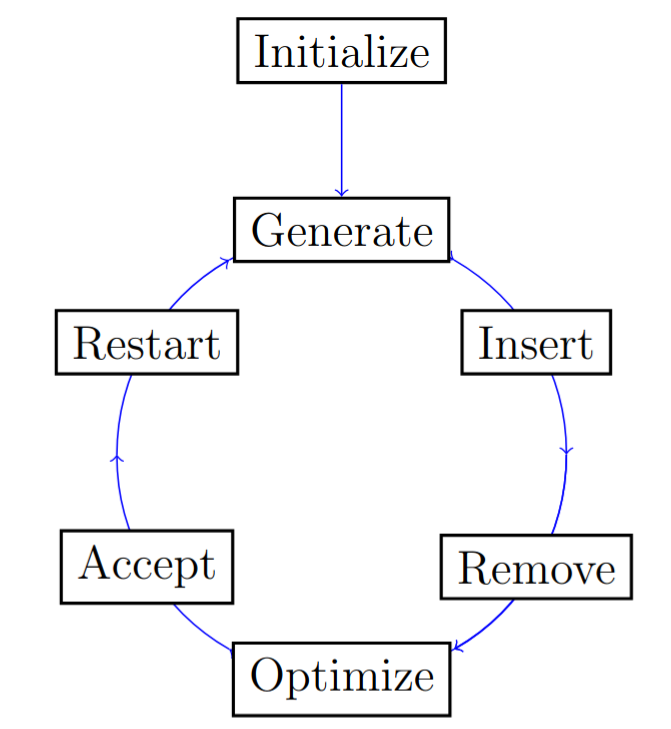
The flow of the CODEX algorithm.