Example scenarios
Fixed structure
This section provides a few examples related to fixed structure designs.
Complete example
The first example is similar to Creating other fixed structure designs in the Quickstart guide. However, it shows the different possible features such as design augmentation, covariates, run level constraints, and evaluation in a single script. The complete Python script is found at example_strip_plot.py.
Mixtures
This example is an example on how to generate mixture experiments for a fixed randomization structure. The complete Python script is found at example_mixture.py. There are two special aspects to generating a design with mixture components.
First, the factors require the type mixture and one mixture component is omitted. For example, below is the code to create a mixture with four components, completely defined by three factors (as the fourth factor is one minus the sum of the other three).
>>> factors = [
>>>     Factor('A', type='mixture', levels=np.arange(0, 1.001, 0.05)),
>>>     Factor('B', type='mixture', levels=np.arange(0, 1.001, 0.05)),
>>>     Factor('C', type='mixture', levels=np.arange(0.2, 0.501, 0.05)),
>>> ]
A mixture factor is a factor with a value between 0 and 1 (which represents a fraction of the total). By default, only the levels 0, 0.5, and 1 are considered, however, by manually specifying the levels, the user can assign minimum and maximum constraints on the mixture component. For example, here, every run requires at least 20% of component C, and at most 50%.
Second, the model is commonly adjusted to a Scheffé-model.
>>> Y2X = mixtureY2X(
>>>     factors,
>>>     mixture_effects=(('A', 'B', 'C'), 'tfi'),
>>> )
Using the mixtureY2X, we can generate a Y2X function
which automatically adds the final mixture component and computes the model. Note that
the function also permits to easily add process variables and any level of cross-terms between
the mixture components and the process variables.
Finally, for export, we can add the fourth mixture component
>>> Y['D'] = 1 - Y.sum(axis=1)
Note
The mixture constraint, indicating the sum of the mixture components cannot be larger than one, is automatically when the algorithm detects mixture components.
An approximated OMARS design (anti-aliasing)
Besides the well-known D-, I- and A-optimality criteria, a new type of designs is emerging: OMARS (orthogonally, minimally aliased response surface designs, Núñez Ares and Goos (2019)). These designs permit to estimate the main effects of a model, but guarantee complete orthogonality (or decorrelation) from the two-factor interactions and quadratic effects. They are anti-aliasing.
The Python script is found at example_approx_omars.py.
While with heuristic algorithms, we cannot guarantee complete orthogonality,
we can optimize for anti-aliasing using the Aliasing
metric. In other words, in this example, we optimize for minimal
covariance between the main effects, and the two-factor interactions and quadratic effects.
To do so, we first specify six factors
>>> factors = [
>>>     Factor('A', type='continuous'),
>>>     Factor('B', type='continuous'),
>>>     Factor('C', type='continuous'),
>>>     Factor('D', type='continuous'),
>>>     Factor('E', type='continuous'),
>>>     Factor('F', type='continuous'),
>>> ]
Next, we require a full response surface model
>>> model = partial_rsm_names({
>>>     'A': 'quad',
>>>     'B': 'quad',
>>>     'C': 'quad',
>>>     'D': 'quad',
>>>     'E': 'quad',
>>>     'F': 'quad',
>>> })
>>> Y2X = model2Y2X(model, factors)
Finally, we specify which covariance we want to minimize
>>> from_aliasing = np.arange(len(factors)+1)
>>> to_aliasing = np.arange(len(model))
The first term in the model is the intercept, followed by the main effects of the factors. Therefore, we specify the from_aliasing as the first seven terms. Next, we want to minimize the aliasing of these main effects to every other element in the matrix, specified by to_aliasing.
Next, we define the weights of these covariances. The weight-matrix has in this case 7 rows, and 28 columns. We more heavily weigh to the main effects and intercept (w1) compared to the other effects in the model (w2).
w1 \(\in \mathcal{R}^{1 \times 1}\) |
w1 \(\in \mathcal{R}^{1 \times n_1}\) |
w2 \(\in \mathcal{R}^{1 \times n_2}\) |
w2 \(\in \mathcal{R}^{1 \times n_1}\) |
w1 \(\in \mathcal{R}^{n_1 \times 1}\) |
w1 \(\in \mathcal{R}^{n_1 \times n_1}\) |
w2 \(\in \mathcal{R}^{n_1 \times n_2}\) |
w2 \(\in \mathcal{R}^{n_1 \times n_1}\) |
with \(n_1=6\) the number of main effects and \(n_2=15\) the number of interaction effects. The first row is from the intercept to the different effects, the second row contains all main effects to the different effects. The first column is to the intercept, the second column to the main effects, the third column to the interaction effects, and the fourth column to the quadratic effects.
>>> n1, n2 = len(factors), len(model)-2*len(factors)-1
>>> w1, w2 = 1/((n1+1)*(n1+1)), 1/((n2+n1)*(n1+1))
>>> W = np.block([
>>>     [ w1 * np.ones(( 1, 1)), w1 * np.ones(( 1, n1)), w2 * np.ones(( 1, n2)), w2 * np.zeros(( 1, n1))], # Intercept
>>>     [ w1 * np.ones((n1, 1)), w1 * np.ones((n1, n1)), w2 * np.ones((n1, n2)), w2 *  np.ones((n1, n1))], # Main effects
>>> ])
Finally, to show that we can completely control the desired aliasing, we can specify that we are only interested in the covariances of the parameter estimates, but not the variances.
>>> W[np.arange(len(W)), np.arange(len(W))] = 0
The final metric is then
>>> metric = Aliasing(effects=from_aliasing, alias=to_aliasing, W=W)
The two typical small covariance bands between the main effects and the other factors are clearly visible.
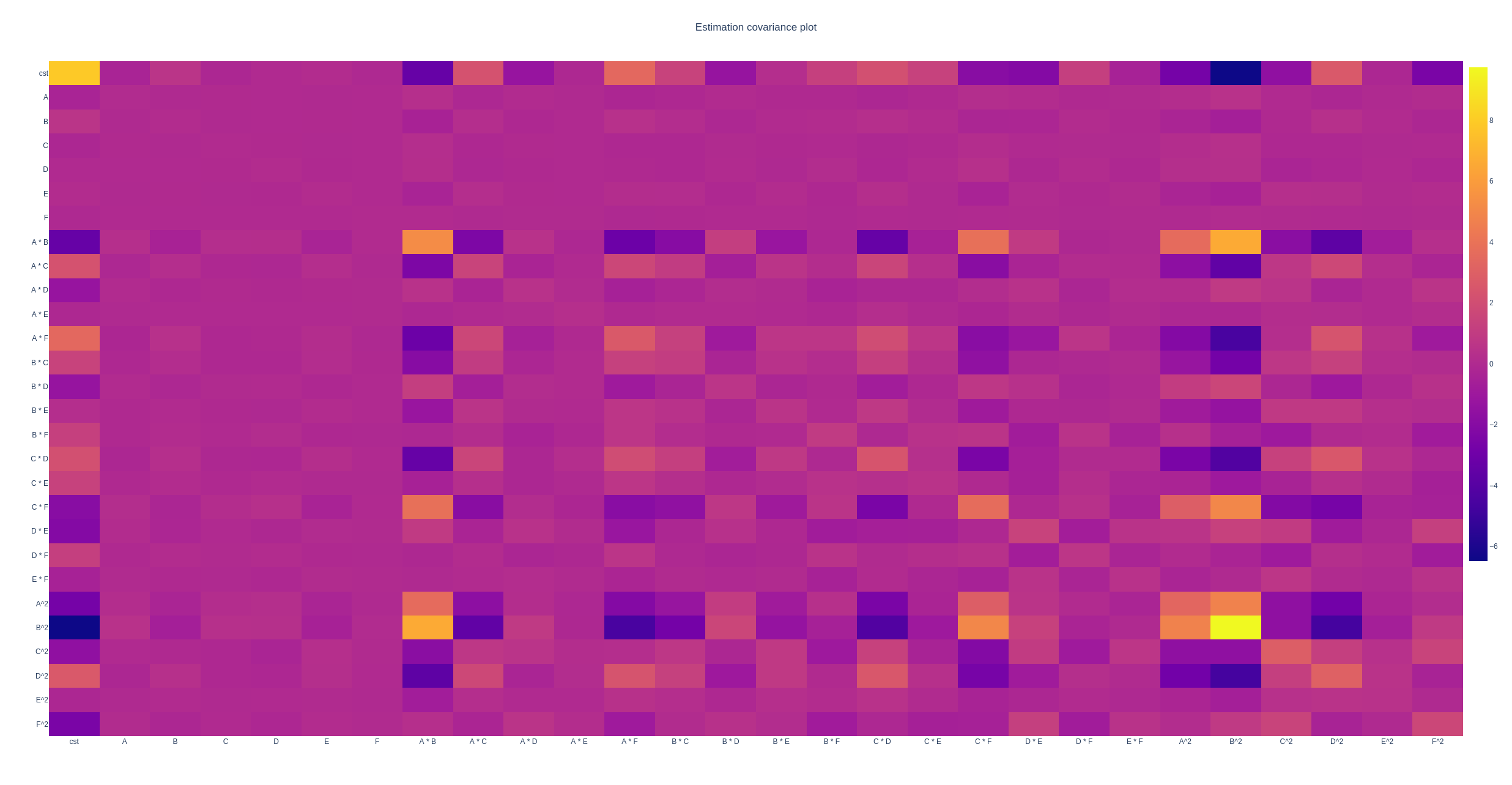
The estimation covariance-matrix of the anti-aliasing experiment.
Complete splitk-plot design
Similar to the first example, this example shows the different features implemented to generate a splitk-plot design. The Python script is found at example_splitk_plot.py.
Splitk-plot design augmentation
Augmentation at the end of the design can easily be done by providing the algorithm with a prior design. The Python script is found at example_splitk_augment.py. For example
>>> prior = (
>>>     pd.DataFrame([
>>>         ['L1', 0, -1],
>>>         ['L1', 1, 1],
>>>         ['L1', -1, 0],
>>>         ['L1', -1, -1],
>>>         ['L2', -1, 0],
>>>         ['L2', 0, 0],
>>>         ['L2', 1, 0],
>>>         ['L2', 0, -1],
>>>     ], columns=['A', 'B', 'C']),
>>>     [Plot(level=0, size=4), Plot(level=1, size=2)]
>>> )
specifies a prior split-plot design with 2 whole plots, and 4 runs per whole plot. To augment the design, we specify the sizes of the new design (including the prior) we want to have. For example
>>> etc = Plot(level=0, size=4)
>>> htc = Plot(level=1, size=8)
specifies we want to generate a split-plot design with 8 whole plots and 4 runs per whole plot. The first two whole plots are already specified by the prior.
Splitk-plot design augmentation in each plot
Sometimes, we do not know how many runs per plot are possible upfront. In such a case, we generally make an estimate and generate the design based on this estimate. If we underestimate the number of runs, there are two options in practice:
Either we regenerate the complete design once we notice more runs per whole plot are feasible
Or, if there is no time, we can generate such an augmentation upfront. For example, if the person who generates the design is unavailable during the experimentation.
In the latter case, we can augment the design by adding one or multiple additional runs to each plot. This approach permits us to have an optimal design in case our estimate is good, and a near-optimal design in case our estimate was bad, without needing to regenerate the design.
The Python script is found at example_splitk_augment_split.py.
Let us consider a prior with 4 whole plots, and 2 runs per whole plot
>>> prior = (
>>>     pd.DataFrame([
>>>         ['L1', 0, -1],
>>>         ['L1', 1, 1],
>>>         ['L2', -1, 0],
>>>         ['L2', 0, 0],
>>>         ['L3', -1, 0],
>>>         ['L3', 1, 1],
>>>         ['L2', 1, -1],
>>>         ['L2', 0, 1],
>>>     ], columns=['A', 'B', 'C']),
>>>     [Plot(level=0, size=2), Plot(level=1, size=4)]
>>> )
meaning we estimate two runs per whole plot to be possible. However, it may be larger, up to four runs per whole plot. We can then specify an augmentation
>>> etc = Plot(level=0, size=4)
>>> htc = Plot(level=1, size=4)
with again four whole plots, but now 4 runs per whole plot. The first two runs of each whole plot will be the prior, the last two are optimized by the algorithm.
Note
We can combine this, and the previous example to extend both the number of runs per whole plot, and the number of whole plots simultaneously.
Splitk-plot design with a predetermined factor
Suppose there is a factor which must be fixed because it requires a certain order in the execution. For example, the hard-to-change factor must first be set to 1, then 0, then -1.
The Python script is found at example_splitk_fixed_factor.py.
We can specify such a design by creating a prior and noting to the algorithm that from this prior, not all levels must be fixed. Some can still be optimized.
Note
The same effect is possible with a covariate function. However, the covariate function is computationally more expensive due to a lack of update formulas, and cannot be included in run level constraints.
Assume we have the following prior
>>> prior = (
>>>     pd.DataFrame([
>>>         ['L1'], ['L1'], ['L1'], ['L1'],
>>>         ['L2'], ['L2'], ['L2'], ['L2'],
>>>         ['L3'], ['L3'], ['L3'], ['L3'],
>>>         ['L2'], ['L2'], ['L2'], ['L2'],
>>>         ['L1'], ['L1'], ['L1'], ['L1'],
>>>         ['L3'], ['L3'], ['L3'], ['L3'],
>>>         ['L1'], ['L1'], ['L1'], ['L1'],
>>>         ['L2'], ['L2'], ['L2'], ['L2'],
>>>     ], columns=['A']).assign(B=0, C=0),
>>>     [Plot(level=0, size=4), Plot(level=1, size=8)]
>>> )
with 8 whole plots, and 4 runs per whole plot. The levels of factor A must be fixed in this order, but the levels of factors B and C can be anything. We create a prior with the correct levels of factor A, and set the levels of factors B and C to zero.
Next, we specify the groups from the prior to be optimized.
>>> grps = [np.array([]), np.arange(nruns), np.arange(nruns)]
Every factor requires a group, which is an array of indices of the groups to be optimized. For example, the first group could have values from 0 up to (not including) 8. If 0 is included in the first array, factor A can be changed in the first group, meaning the first four rows in this scenario. However, as factor A should be fixed, we specify an empty array indicating no group can be optimized. The easy-to-change factors B and C can have indices from 0 up to 8*4 = 32. We specify all as none should be fixed.
Finally, we specify an overall design of the same size
>>> etc = Plot(level=0, size=4)
>>> htc = Plot(level=1, size=8)
Cost-optimal
This section provides a few examples related to the cost optimal designs.
Complete CODEX example
The first example is similar to An example (CODEX) in the Quickstart guide. However, it shows the different possible features such as design augmentation, covariates, run level constraints, and evaluation in a single script. The Python script is found at example_codex.py.
Mixtures
This example is an example on how to generate mixture experiments for a fixed randomization structure. The complete Python script is found at example_mixture.py. There are two special aspects to generating a design with mixture components.
First, the factors require the type mixture and one mixture component is omitted. For example, below is the code to create a mixture with three components, completely defined by two factors (as the third factor is one minus the sum of the other two).
>>> factors = [
>>>     Factor('A', type='mixture', grouped=False, levels=np.arange(0, 1.0001, 0.05)),
>>>     Factor('B', type='mixture', grouped=False, levels=np.arange(0, 1.0001, 0.05)),
>>> ]
A mixture factor is a factor with a value between 0 and 1 (which represents a fraction of the total). By default, only the levels 0, 0.5, and 1 are considered, however, by manually specifying the levels, the user can specify minimum and maximum constraints on the mixture component. For an example, see Mixtures.
Second, the model is commonly adjusted to a Scheffé-model.
>>> Y2X = mixtureY2X(
>>>     factors,
>>>     mixture_effects=(('A', 'B'), 'tfi'),
>>> )
Using the mixtureY2X, we can generate a Y2X function
which automatically adds the final mixture component and computes the model. Note that
the function also permits to easily add process variables and any level of cross-terms between
the mixture components and the process variables.
Finally, for export, we can add the fourth mixture component
>>> Y['D'] = 1 - Y.sum(axis=1)
Note
The mixture constraint, indicating the sum of the mixture components cannot be larger than one, is automatically when the algorithm detects mixture components.
The cost depends on the magnitude of the change in a factor’s level
What if the transition cost depends on the magnitude of the transition? For example, heating an oven from 0°C to 100°C requires more time than heating it to 50°C. Accounting for this transition is only possible with cost-optimal designs which determine the structure of the design automatically.
The Python script is found at example_scaled.py.
Let us specify an experiment with two hard-to-change factors A and B, and two easy-to-change factors C and D
>>> factors = [
>>>     Factor('A', type='continuous', min=2, max=5),
>>>     Factor('B', type='continuous'),
>>>     Factor('E', type='continuous', grouped=False),
>>>     Factor('F', type='continuous', grouped=False),
>>> ]
We can specify a scaled transition cost using the
scaled_parallel_worker_cost or
scaled_single_worker_cost functions.
Each transition cost is specified as a tuple of four elements, of which, for now, we consider the first two and
the last two to be the same. A complete example is in The cost depends on the magnitude and direction of the change in a factor’s level.
The general transition cost of a scaled scenario is specified as \(a + b \cdot mag\), with a the base cost, b the scaling term, and mag the magnitude of the transition. The base cost is specified in the first two elements of the tuple. The scaling term, from the minimum to the maximum, is specified in the latter two elements of the tuple.
In this example, factor A has a scaled cost with no base cost. The time to go from the minimum to the maximum is two hours. Factor B has a fixed reset cost of one hour. Finally, the easy-to-change factors (which are reset with every run) require one minute to reset. There is also an experiment execution time of five minutes. The total transition time is determined by the most-hard-to-change factor as specified in An example (CODEX).
>>> max_transition_cost = 3*4*60
>>> transition_costs = {
>>>     'A': (0, 0, 2*60, 2*60), # From -1 to +1, scaled in between, no base cost
>>>     'B': (60, 60, 0, 0), # Constant transition cost
>>>     'E': (1, 1, 0, 0), # Constant transition cost
>>>     'F': (1, 1, 0, 0), # Constant transition cost
>>> }
>>> execution_cost = 5
>>>
>>> cost_fn = scaled_parallel_worker_cost(
>>>     transition_costs, factors,
>>>     max_transition_cost, execution_cost
>>> )
The cost depends on the magnitude and direction of the change in a factor’s level
What if the cost not only depends on the magnitude, but also the direction? Heating an oven from 0°C to 100°C takes longer than heating it to 50°C. On top, cooling is even slower because there is an active heating element, but no active cooling element in the oven. In such a scenario, the cost depends on the magnitude, but also the direction of the change. There is an asymmetry in the cost function.
The Python script is found at example_asymmetric.py.
Let us again specify an experiment with two hard-to-change factors A and B, and two easy-to-change factors C and D
>>> factors = [
>>>     Factor('A', type='continuous', min=2, max=5),
>>>     Factor('B', type='continuous'),
>>>     Factor('E', type='continuous', grouped=False),
>>>     Factor('F', type='continuous', grouped=False),
>>> ]
We use the same cost function as in The cost depends on the magnitude of the change in a factor’s level, however, now we require all four elements of the tuple. The tuple defines:
The base cost in the positive direction (heating, from minimum to maximum)
The base cost in the negative direction (cooling, from maximum to minimum)
The scale in the positive direction
The scale in the negative direction
In this example, it takes one hour to go from the minimum to the maximum, and two hours to go from the maximum back to the minimum. There is also an execution cost of five minutes.
>>> max_transition_cost = 3*4*60
>>> transition_costs = {
>>>     'A': (0, 0, 1*60, 2*60), # Positive change is 1 hour, negative is 2 hours
>>>     'B': (60, 60, 0, 0), # Constant transition cost
>>>     'E': (1, 1, 0, 0), # Constant transition cost
>>>     'F': (1, 1, 0, 0), # Constant transition cost
>>> }
>>> execution_cost = 5
>>>
>>> cost_fn = scaled_parallel_worker_cost(
>>>     transition_costs, factors,
>>>     max_transition_cost, execution_cost
>>> )