Customization
Custom model
See Custom models for more information.
Custom categorical encoding
See Custom categorical encoding for more information.
Custom regressors
To create your own regressor, create a new class extending the
RegressionMixin
for single model regressors, and
MultiRegressionMixin
for regressors outputting multiple models. These mixins automatically
extend the sklearn interfaces so that you can also use them in their pipelines.
>>> class MyRegressor(RegressionMixin):
>>>     def _fit(self, X, y):
>>>         # Your fit code
>>>         pass
>>>
>>>     def _predict(self, X):
>>>         # Optional, if you require a custom prediction
>>>         # Defaults to
>>>         return np.sum(X[:, self.terms_] * np.expand_dims(self.coef_, 0), axis=1) \
>>>                       * self.y_std_ + self.y_mean_
One function must be implemented:
_fit which takes
the encoded and normalized model matrix of the data, X, and the normalized
outputs, y. See the RegressionMixin
documentation for more information about which other parameters are available
during fitting and model selection. If desired, the user could overwrite the default
_predict,
however, maybe the other attributes and functions must also be updated.
Note
It is important that the constructor of the regressor only sets the variables,
and not adjust or validate them. Validation and any adjustments should be done
during fitting in the
_regr_params,
_compute_derived
and _validate_X.
During fitting, certain attributes must be set. For
RegressionMixin,
the user must set (all parameters are also indicated as the attributes of the mixin):
terms_ : a 1-D numpy integer array with the indices of the selected terms in the encoded model matrix.
coef_ : the coefficients of the terms for a normalized model matrix.
scale_ : the scale (or variance of the random errors) of the data.
vcomp_ : a 1-D numpy floating point arry with the estimated variance components in a mixed model.
fit_ : optionally the fit object, returned by fit_fn_. If specified, the used can call .summary() which is forwarded here.
Have a look at the source code of
SimpleRegressor for a
simple example.
For a MultiRegressionMixin,
only three attributes must be set:
models_ : A list of 1-D numpy integer arrays, similar to terms_ above. The models should be sorted by the selection metric, maximum first.
selection_metrics_ : The values of the selection metric as a 1-D numpy floating point array. a higher selection metric indicates a better model.
metric_name_ : The name of the selection metric as a string. Used for interpretation.
Simulated annealing model selection (SAMS)
Simulated annealing model selection, or SAMS, was devised by Wolters and Bingham (2012). It is a model selection algorithm, which instead of looking at the statistical significance, like is most commonly used, simulates multiple models and looks at what the good fitting models have in common. The algorithm works in three stages:
The simulation stage: here the algorithm simulates many models of a fixed size using simulated annealing, and sorts them by their \(R^2\). Commonly it simulates 10000 or 20000 models, however it depends on the problem at hand.
The reduction stage: here the algorithm takes the simulated models and looks what the most common 1-factor, 2-factor, 3-factor, etc. combinations are. In other words, it looks at which submodel of size k occurs most frequently in the good fitting models for multiple values of k.
The selection stage: here the algorithm takes the most occuring submodels of each size and compares them to determine an ordering. The ordering is based on the entropy which is explained later.
As you may notice, the algorithm does not output just one model. It outputs multiple models, ordered by which model it has the most confidence in. The last two stages of the algorithm use the result of the first stage to automatically determine an ordering, however, the user may also manually look at a raster plot of the results which looks as follows:
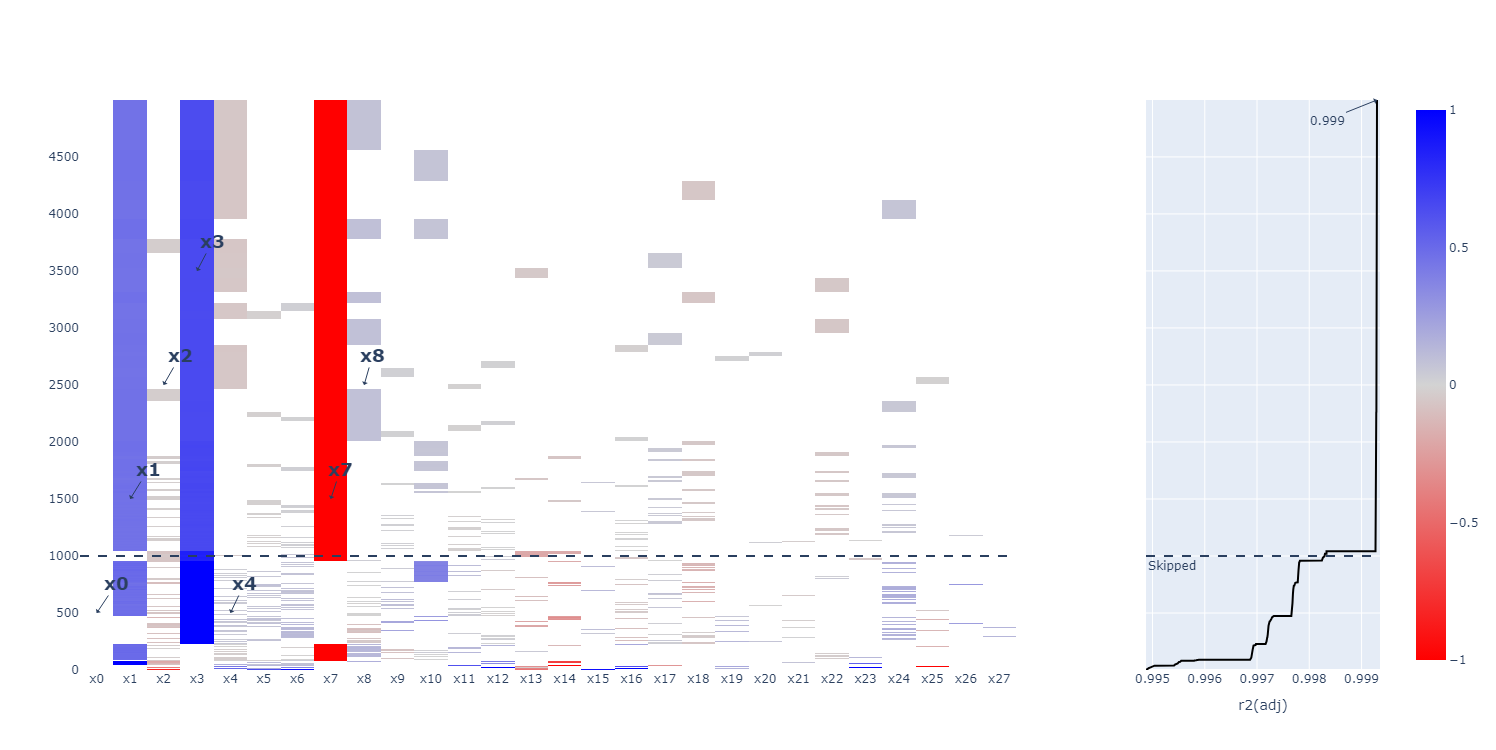
Each row is a model, each column is a potential term in the model, and the color indicates the coefficient of the term. This means that any term not in the model has a coefficient of zero, which is plotted in white. By looking at largely colored columns, we can determine which submodels occur most often (here \(x_1\), \(x_3\) and \(x_7\)).
Note
In some events, multiple distinct models may perform equally well. Such a scenario is difficult to detect in the raster plot, and also by the entropy criterion. Luckily, we can also cluster the results in the raster plot making them more visible. The different terms in each model are binary encoded if the effect is present or not. On this representation, a kmeans clustering is run. This technique was also devised by Wolters and Bingham (2012).
See SamsRegressor for information
on the parameters.
Entropy calculations
The entropy is the most effective addition of the algorithm to perform automated model selection. The entropy is computed as
where \(f_{o}\) is the observed frequency of the submodel in the simulation phase, and \(f_{t}\) is the theoretical frequency this submodel would occur when randomly sampling hereditary models.
In Wolters and Bingham (2012), the authors performed some simulations on screening designs for different model selection algorithms. The oracle method requires prior knowledge about the true model, and each term is tested for significance. The AICc method is Akaike’s Information Criterion (corrected). The authors noted that a search through the hereditary models was performed, from which the best according to the AICc was selected. This, together with the Bayes Information Criterion (BIC) is commonly applied in practice. The last method is the new SAMS method with entropy selection.
Method |
Correct |
Underfitted |
Overfitted |
(Partialy) Wrong |
Oracle |
62.8 |
37.2 |
0 |
0 |
AICc |
7.2 |
0.7 |
53.8 |
38.3 |
SAMS |
43.3 |
16.2 |
15.8 |
24.7 |
The SAMS method with entropy significantly outperforms any other method with 43.3% of models found to be correct. In addition, the oracle method, which has prior knowledge about the true model, also only found 62.8% of the models. AICc only found about 7.2% of the models making it not very suitable for this scenario.
There is one downside to the entropy criterion. Only in the specific case where the model
is a (partial) response surface model with weak heredity can \(f_{t}\)
be computed exactly. To make sure the algorithm is generic enough, a fallback was implemented
to compute an approximation of the entropy using a model sampler. Three different
samplers are implemented:
sample_model_dep_onebyone,
sample_model_dep_mcmc
and sample_model_dep_random.
For each of these samplers, we ran similar simulations to Wolters and Bingham (2012). We start from a PB12 design (Plackett-Burman). Next, we generate a random hereditary model by sampling 1 to 4 main effects, \(n_{main}\), and sequentially sampling \(4 - n_{main}\) interaction effects. Note that this is a weak heredity submodel of a partial response surface design where each factor has linear effects and two-factor interactions.
The results are
Method |
Correct |
Underfitted |
Overfitted |
(Partialy) Wrong |
Exact entropy |
43.7 |
30.3 |
10.5 |
15.5 |
One-by-one |
37.3 |
12.6 |
23.8 |
26.3 |
Markov-chain Monte carlo (mcmc) |
38.8 |
12.3 |
23.3 |
25.6 |
Random |
36.8 |
10.1 |
26.1 |
27.0 |
The first row is the exact entropy method as used in Wolters and Bingham (2012). Note that all three samplers, even though they perform worse than the exact entropy based on the percentage of correct models, still perform significantly better than AICc. When loosening the classification by also classifying models underfitted or overfitted by one term as correct, the exact entropy method has 61.1% accuracy, the one-by-one has 59.1%, the mcmc has 59.3%, and the random has 56.5%. Only a 2% difference for the one-by-one and mcmc samplers.
By default, the one-by-one sampler is used as it performs almost equally as good as the mcmc method, but computes faster.
Warning
The implementation of SAMS uses the samplers by default, however, the exact method
may be used by specifying the entropy_model_order parameter in
SamsRegressor.
However, a large warning should be given to this parameter as it comes with certain
assertions (which are covered in many, but not all scenarios).
First, the heredity mode must be ‘weak’, otherwise the sampling method is still
applied. Second, the model must be generated using
partial_rsm_names followed by
model2Y2X. Third, the factors must
be ordered: first all factors which can have a quadratic effect, second
all factors which can not have quadratic effects, but can have two-factor interactions,
and third all factors which can only have a main effect. Finally, the dependency
matrix must be generated using
order_dependencies.
As an example. Create three factors
>>> factors = [
>>>   Factor('A'), Factor('B'), Factor('C')
>>> ]
Next, create the model orders. The order of the factor names in the dictionary must be the same as those in the list of factors. They also must be ordered quad - tfi - lin.
>>> entropy_model_order = {'A': 'quad', 'B': 'tfi', 'C': 'lin'}
Create the model using partial_rsm_names.
Note that the quad elements are first, then the tfi, and finally the lin elements.
The dictionary parameters must be in the same order as the factors.
>>> model = partial_rsm_names(entropy_model_order)
>>> Y2X = model2Y2X(model, factors)
Next, create the dependencies from the model
>>> dep = order_dependencies(model, factors)
Finally, we can fit SAMS using the exact entropy formula
>>> regr = SamsRegressor(
>>>     factors, Y2X,
>>>     mode='weak', dependencies=dep,
>>>     forced_model=np.array([0], np.int\_),
>>>     entropy_model_order=entropy_model_order
>>> )