Example scenarios
Dropping based on p-values
A common strategy is to fit a very large model and drop terms one by one based on their p-value significance. Similar to the quickstart, we will fit a response surface model with three continuous variables. The full Python script is found at drop_pvalue.py.
Start with the imports
>>> import numpy as np
>>> import pandas as pd
>>>
>>> from pyoptex.utils import Factor
>>> from pyoptex.utils.model import model2Y2X, order_dependencies, partial_rsm_names
>>> from pyoptex.analysis import PValueDropRegressor
>>> from pyoptex.analysis.utils.plot import plot_res_diagnostics
Define the factors
>>> factors = [
>>>     Factor('A'), Factor('B'), Factor('C')
>>> ]
Generate the random simulation data. The true model in our case is \(y = 5 + 2*A + 3*C - 4*A*B + \epsilon\).
>>> # The number of random observations
>>> N = 200
>>>
>>> # Define the data
>>> data = pd.DataFrame(np.random.rand(N, 3) * 2 - 1, columns=[str(f.name) for f in factors])
>>> data['Y'] = 2*data['A'] + 3*data['C'] - 4*data['A']*data['B'] + 5\
>>>                 + np.random.normal(0, 1, N)
Next, we create the response surface model, which contains all potential terms we wish to investigate.
>>> model = partial_rsm_names({str(f.name): 'quad' for f in factors})
>>> Y2X = model2Y2X(model, factors)
Then we need to decide on the model constraints. There are three types of models:
No heredity: This means any term can occur in the model, without any restrictions.
Weak heredity: This means that if a term such as \(A \times B\) occurs in the model, either \(A\), \(B\), or both must also occur in the model. Similar for \(A^2\) to occur, \(A\) must also be in the model.
Strong heredity: Extends weak heredity by forcing that when \(A \times B\) is in the model, both \(A\) and \(B\) must occur.
All these dependencies can be represented by a dependency matrix. This matrix has the same number of rows and columns as there are terms (in the encoded model). Term i depends on term j if dep(i, j) = true.
An easy method to create such a dependency matrix from a generic model is
order_dependencies.
>>> dependencies = order_dependencies(model, factors)
Finally, we fit the regressor on the data using weak heredity and a threshold for the p-value of 5%.
>>> regr = PValueDropRegressor(
>>>     factors, Y2X,
>>>     threshold=0.05, dependencies=dependencies, mode='weak'
>>> )
>>> regr.fit(data.drop(columns='Y'), data['Y'])
Once fitted, we can display the summary of the fit
>>> print(regr.summary())
                            OLS Regression Results
==============================================================================
Dep. Variable:                      y   R-squared:                       0.848
Model:                            OLS   Adj. R-squared:                  0.845
Method:                 Least Squares   F-statistic:                     363.6
Date:                Tue, 07 Jan 2025   Prob (F-statistic):           8.43e-80
Time:                        10:50:08   Log-Likelihood:                -95.613
No. Observations:                 200   AIC:                             199.2
Df Residuals:                     196   BIC:                             212.4
Df Model:                           3
Covariance Type:            nonrobust
==============================================================================
                 coef    std err          t      P>|t|      [0.025      0.975]
------------------------------------------------------------------------------
const          0.0734      0.028      2.619      0.010       0.018       0.129
x1             0.7703      0.048     15.933      0.000       0.675       0.866
x2             1.1347      0.046     24.525      0.000       1.043       1.226
x3            -1.5286      0.082    -18.645      0.000      -1.690      -1.367
==============================================================================
Omnibus:                        1.348   Durbin-Watson:                   1.859
Prob(Omnibus):                  0.510   Jarque-Bera (JB):                1.233
Skew:                           0.192   Prob(JB):                        0.540
Kurtosis:                       2.995   Cond. No.                         2.96
==============================================================================
Or the prediction formula. Note that indeed the correct model was selected in this case.
>>> print(regr.model_formula(model=model))
0.073 * cst + 0.770 * A + 1.135 * C + -1.529 * A * B
Predicting remains the same
>>> data['pred'] = regr.predict(data.drop(columns='Y'))
Just like the residual diagnostics
>>> plot_res_diagnostics(
>>>     data, y_true='Y', y_pred='pred',
>>>     textcols=[str(f.name) for f in factors],
>>> ).show()
In some cases, the user is interested in strong heredity models. However, forcing strong heredity during the model selection process often puts too much pressure on the main effects, meaning the interactions are often missed. Besides forcing strong heredity, we could force weak heredity instead and transform the final model to a strong heredity model.
Instead of simply predicting based on the regr, we can transform the result to a strong model
>>> terms_strong = model2strong(regr.terms_, dependencies)
>>> model = model.iloc[terms_strong]
>>> Y2X = model2Y2X(model, factors)
And fit a simple model
>>> regr_simple = SimpleRegressor(factors, Y2X).fit(data.drop(columns='Y'), data['Y'])
The full Python script can be found at drop_pvalue_strong.py.
Mixed linear model
Mixed models occur very often when having hard-to-change factors. Every result from a split-plot design, split-split-plot design, strip-plot design, staggered-level design, etc. should be modelled by a mixed model. The Zs must be specified in the dataframe to use random effects. Similar to the quickstart, we will fit a response surface model with three continuous variables. The full Python script is found at simple_model_mixedlm.py.
Start with the imports
>>> import numpy as np
>>> import pandas as pd
>>>
>>> from pyoptex.utils import Factor
>>> from pyoptex.utils.model import model2Y2X, partial_rsm_names
>>> from pyoptex.analysis import SimpleRegressor
>>> from pyoptex.analysis.utils.plot import plot_res_diagnostics
Create the factors
>>> factors = [
>>>     Factor('A'), Factor('B'), Factor('C')
>>> ]
Generate random simulation data. We also generate a random effect to show the mixed modelling. Five groups will be made, spaced over 200 ovbservations.
>>> # The number of random observations
>>> N = 200
>>> nre = 5
>>>
>>> # Define the data
>>> data = pd.DataFrame(np.random.rand(N, 3) * 2 - 1, columns=[str(f.name) for f in factors])
>>> data['RE'] = np.array([f'L{i}' for i in range(nre)])[np.repeat(np.arange(nre), N//nre)]
>>> data['Y'] = 2*data['A'] + 3*data['C'] - 4*data['A']*data['B'] + 5\
>>>                 + np.random.normal(0, 1, N)\
>>>                 + np.repeat(np.random.normal(0, 1, nre), N//nre)
Similar to the quickstart, we create the response surface model
>>> model = partial_rsm_names({str(f.name): 'quad' for f in factors})
>>> Y2X = model2Y2X(model, factors)
Then we fit the mixed model by specifying the column ‘RE’ in the data as the random effect. Each random effect column is intepreted as a categorical column (with strings).
>>> # Define random effects
>>> random_effects = ('RE',)
>>>
>>> # Create the regressor
>>> regr = SimpleRegressor(factors, Y2X, random_effects)
>>> regr.fit(data.drop(columns='Y'), data['Y'])
Once fitted, we can display the summary of the fit
>>> print(regr.summary())
         Mixed Linear Model Regression Results
========================================================
Model:            MixedLM Dependent Variable: y
No. Observations: 200     Method:             REML
No. Groups:       1       Scale:              0.1408
Min. group size:  200     Log-Likelihood:     -109.1928
Max. group size:  200     Converged:          Yes
Mean group size:  200.0
--------------------------------------------------------
        Coef.   Std.Err.     z     P>|z|  [0.025  0.975]
--------------------------------------------------------
const    0.084     0.193    0.438  0.662  -0.293   0.462
x1       0.716     0.048   14.992  0.000   0.622   0.809
x2      -0.049     0.045   -1.085  0.278  -0.137   0.039
x3       1.073     0.045   23.981  0.000   0.985   1.161
x4      -1.420     0.080  -17.761  0.000  -1.577  -1.263
x5      -0.081     0.082   -0.986  0.324  -0.242   0.080
x6       0.001     0.074    0.011  0.991  -0.144   0.146
x7       0.014     0.092    0.151  0.880  -0.166   0.194
x8      -0.065     0.089   -0.734  0.463  -0.240   0.109
x9       0.017     0.088    0.197  0.844  -0.155   0.189
g0 Var   0.166     0.324
========================================================
Print the prediction formula on the encoded, normalized model matrix.
See model_formula
for more information.
>>> print(regr.model_formula(model=model))
0.084 * cst + 0.716 * A + -0.049 * B + 1.073 * C + -1.420 * A * B + -0.081 * A * C + 0.001 * B * C + 0.014 * A^2 + -0.065 * B^2 + 0.017 * C^2
Predicting is still the same.
>>> data['pred'] = regr.predict(data.drop(columns='Y'))
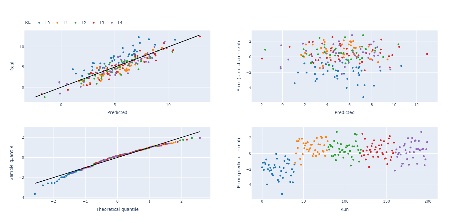
When plotting the residual diagnostics, we can also indicate the random effect groups with a color.
>>> plot_res_diagnostics(
>>>     data, y_true='Y', y_pred='pred',
>>>     textcols=[str(f.name) for f in factors],
>>>     color='RE'
>>> ).show()
Simulated Annealing Model Selection (SAMS)
While model selection is often performed based on p-values or metrics such as the AICc or BIC, SAMS improves on most of them. For more extensive information on the algorithm, see Simulated annealing model selection (SAMS).
In this example, we have six factors, A through F, and wish to detect the weak heredity model \(A + C + A \times B\). The full Python script is at sams_generic.py.
First, the imports
>>> import numpy as np
>>> import pandas as pd
>>>
>>> from pyoptex.utils import Factor
>>> from pyoptex.utils.model import model2Y2X, order_dependencies, partial_rsm_names
>>> from pyoptex.analysis import SamsRegressor
>>> from pyoptex.analysis.utils.plot import plot_res_diagnostics
Next, we define the factors and simulate some data.
>>> # Define the factors
>>> factors = [
>>>     Factor('A'), Factor('B'), Factor('C'),
>>>     Factor('D'), Factor('E'), Factor('F'),
>>> ]
>>>
>>> # The number of random observations
>>> N = 200
>>>
>>> # Define the data
>>> data = pd.DataFrame(np.random.rand(N, len(factors)) * 2 - 1, columns=[str(f.name) for f in factors])
>>> data['Y'] = 2*data['A'] + 3*data['C'] - 4*data['A']*data['B'] + 5\
>>>                 + np.random.normal(0, 1, N)
Then, as in any analysis, we define the Y2X function, which is a full response surface model, and the corresponding heredity dependencies.
>>> # Create the model
>>> model_order = {str(f.name): 'quad' for f in factors}
>>> model = partial_rsm_names(model_order)
>>> Y2X = model2Y2X(model, factors)
>>>
>>> # Define the dependencies
>>> dependencies = order_dependencies(model, factors)
Finally, we fit the SAMS model
>>> regr = SamsRegressor(
>>>     factors, Y2X,
>>>     dependencies=dependencies, mode='weak',
>>>     forced_model=np.array([0], np.int64),
>>>     model_size=6, nb_models=5000, skipn=1000,
>>> )
>>> regr.fit(data.drop(columns='Y'), data['Y'])
Note
By specifying the entropy_model_order parameter in the
SamsRegressor,
we can use the exact entropy caluclations. For more information,
see Entropy calculations. The full Python script is at
sams_partial_rsm.py.
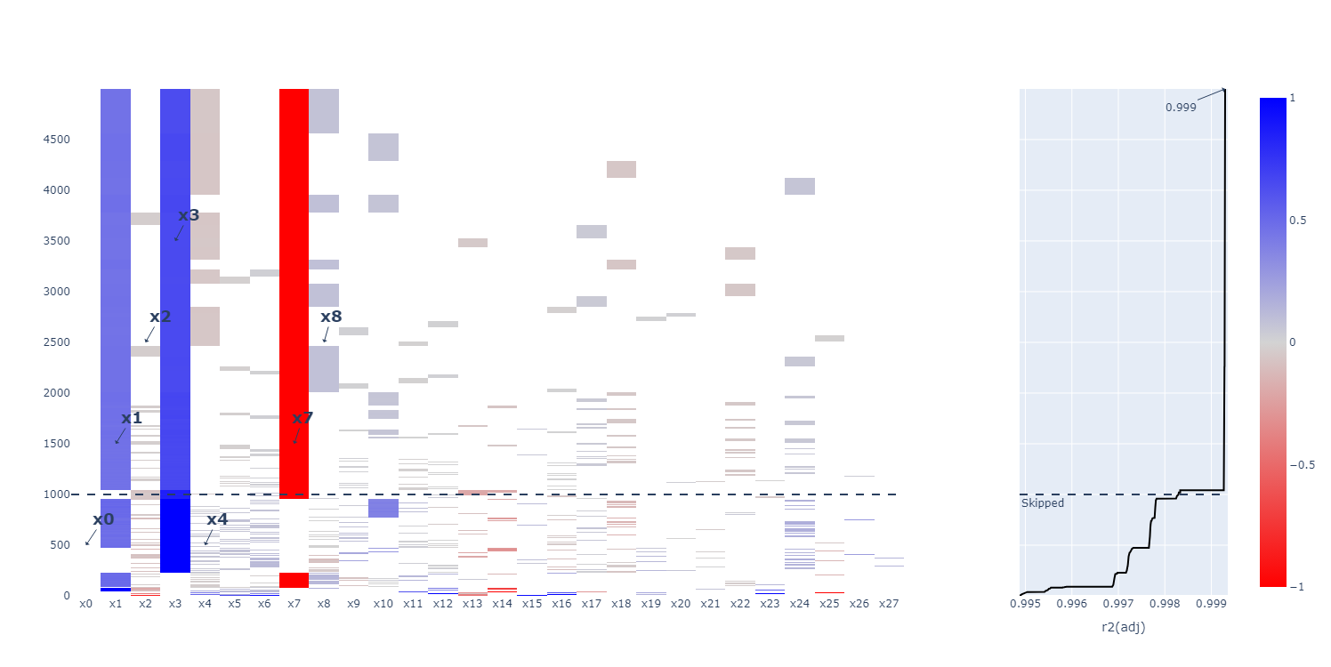
Finally, we can analyze the generated models. To manually extract a model, use
the plot_selection
function.
>>> regr.plot_selection().show()
SamsRegressor
is a MultiRegressionMixin,
meaning it finds multiple good-fitting models and orders them. By default, the best
can be analyzed as before
>>> # Print the summary
>>> print(regr.summary())
                            OLS Regression Results
==============================================================================
Dep. Variable:                      y   R-squared:                       0.858
Model:                            OLS   Adj. R-squared:                  0.856
Method:                 Least Squares   F-statistic:                     394.5
Date:                Tue, 07 Jan 2025   Prob (F-statistic):           9.15e-83
Time:                        15:23:33   Log-Likelihood:                -88.642
No. Observations:                 200   AIC:                             185.3
Df Residuals:                     196   BIC:                             198.5
Df Model:                           3
Covariance Type:            nonrobust
==============================================================================
                 coef    std err          t      P>|t|      [0.025      0.975]
------------------------------------------------------------------------------
const         -0.0043      0.027     -0.159      0.874      -0.058       0.049
x1             0.8045      0.048     16.689      0.000       0.709       0.900
x2             1.1409      0.045     25.356      0.000       1.052       1.230
x3            -1.7373      0.084    -20.769      0.000      -1.902      -1.572
==============================================================================
Omnibus:                        1.979   Durbin-Watson:                   2.166
Prob(Omnibus):                  0.372   Jarque-Bera (JB):                1.934
Skew:                          -0.238   Prob(JB):                        0.380
Kurtosis:                       2.932   Cond. No.                         3.17
==============================================================================
Or
>>> # Print the formula in encoded form
>>> print(regr.model_formula(model=model))
-0.004 * cst + 0.805 * A + 1.141 * C + -1.737 * A * B
Prediction is still the same.
>>> data['pred'] = regr.predict(data.drop(columns='Y'))
And the residual plot of the highest entropy model can be found using
>>> plot_res_diagnostics(
>>>     data, y_true='Y', y_pred='pred',
>>>     textcols=[str(f.name) for f in factors],
>>> ).show()
Note
If the best model is not the desired model, you can extract any other model
in the list by accessing models_
after fitting. These are ordered by highest entropy first.
Once you selected a model, you can refit it, similar to the p-value example. Instead of simply predicting based on the regr, we can select the desired model
>>> terms = regr.models_[i]
>>> model = model.iloc[terms]
>>> Y2X = model2Y2X(model, factors)
And fit a simple model
>>> regr_simple = SimpleRegressor(factors, Y2X).fit(data.drop(columns='Y'), data['Y'])